Modulations
Modulation is the procedure of changing signal parameters to make it more suitable for transmission in communication systems. The information from modulation signal \(\boldsymbol{u_m}\) is being packed into carrier signal \(\boldsymbol{u_c}\), thus changing it’s properties and obtaining the modulated signal \(\boldsymbol{u}\). Although the choice of signals can be arbitrary, most common choice for carrier signal is sinusoidal function \(u_c = U_c cos(\omega_c t)\). Modulation causes the frequency translation of the modulation signal from baseband to the frequency band of the carrier signal. After the transfer over communication channel, information is unpacked at receiver side in the process called demodulation. By the property of carrier signal which is impacted by modulation, we differentiate these modulation types:
- Amplitude modulation:
Changing the amplitude of carrier signal around the mean value. Change is proportional to the modulation signal with proportionality constant called modulation index \(K_a\).
\[u = (U_c + K u_m) cos(\omega_c t)\]- Phase modulation:
Varying the instantaneous phase of the carrier signal proportional to the modulation signal with proportionality constant \(K_p\)
\[u = U_c cos(\omega_c t + K_p u_m)\]- Frequency modulation:
Varying the instantaneous frequency of the carrier signal proportional to the modulation signal with proportionality constant \(K_\omega\)
\[u = U_c cos(\omega_c t + K_\omega \int_{0}^{t} u_m \,dt)\]
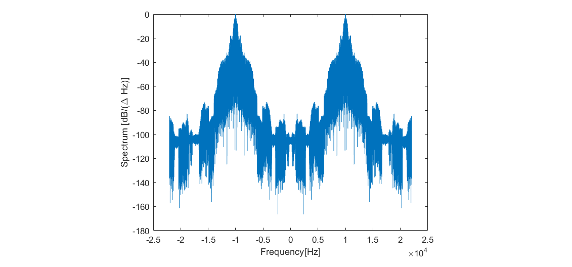
Fig. 1. Spectrum of an amplitude-modulated signal.
Discrete Modulations
Modulating the sinusoidal carrier with discrete signals creates the symbols which represents some digital binary value. Symbols are parts of the sinusoidal signal which differ in amplitude, frequency or phase. In order to prevent interference of the symbols and prevent detection errors, they have be created from orthogonal basis functions. Two functions \(\phi_i\) and \(\phi_j\) are orthogonal if
Equals \(0\) for \(i \ne j\), and \(1\), for \(i = j\). Here \(T_s\) represents the duration of the symbol. Symbols are generated as \(s = s(i) \phi_i + s(j) \phi_j\). Energy of the symbol is given as:
Plot of the symbols \(s\) in \(\phi_i, \phi_j\) basis is called constellation. Each symbol \(s\) can represent one bit (then it is called binary modulation) or more bits. To simplify the expressions, we chose the values \(T_s = E_s = 1\).
- Amplitude shift keying (ASK):
\(\phi_1 = cos(2 \pi f t)\)
1: \(s_1 = 1\cdot\phi_1 = cos(2 \pi f t)\)
0: \(s_0 = 0\cdot\phi_1 = 0\)
- Phase shift keying (PSK):
\(\phi_1 = cos(2 \pi f t)\)
1: \(s_1 = 1\cdot\phi_1 = cos(2 \pi f t)\)
0: \(s_0 = -1\cdot\phi_1 = -cos(2 \pi f t)\)
- Frequency shift keying (FSK):
\(\phi_1 = cos(2 \pi f_1 t), \phi_2 = cos(2 \pi f_2 t)\)
1: \(s_1 = 1\cdot\phi_1 + 0\cdot\phi_2 = cos(2 \pi f_1 t)\)
0: \(s_0 = 0\cdot\phi_1 + 1\cdot\phi_2 = cos(2 \pi f_2 t)\)
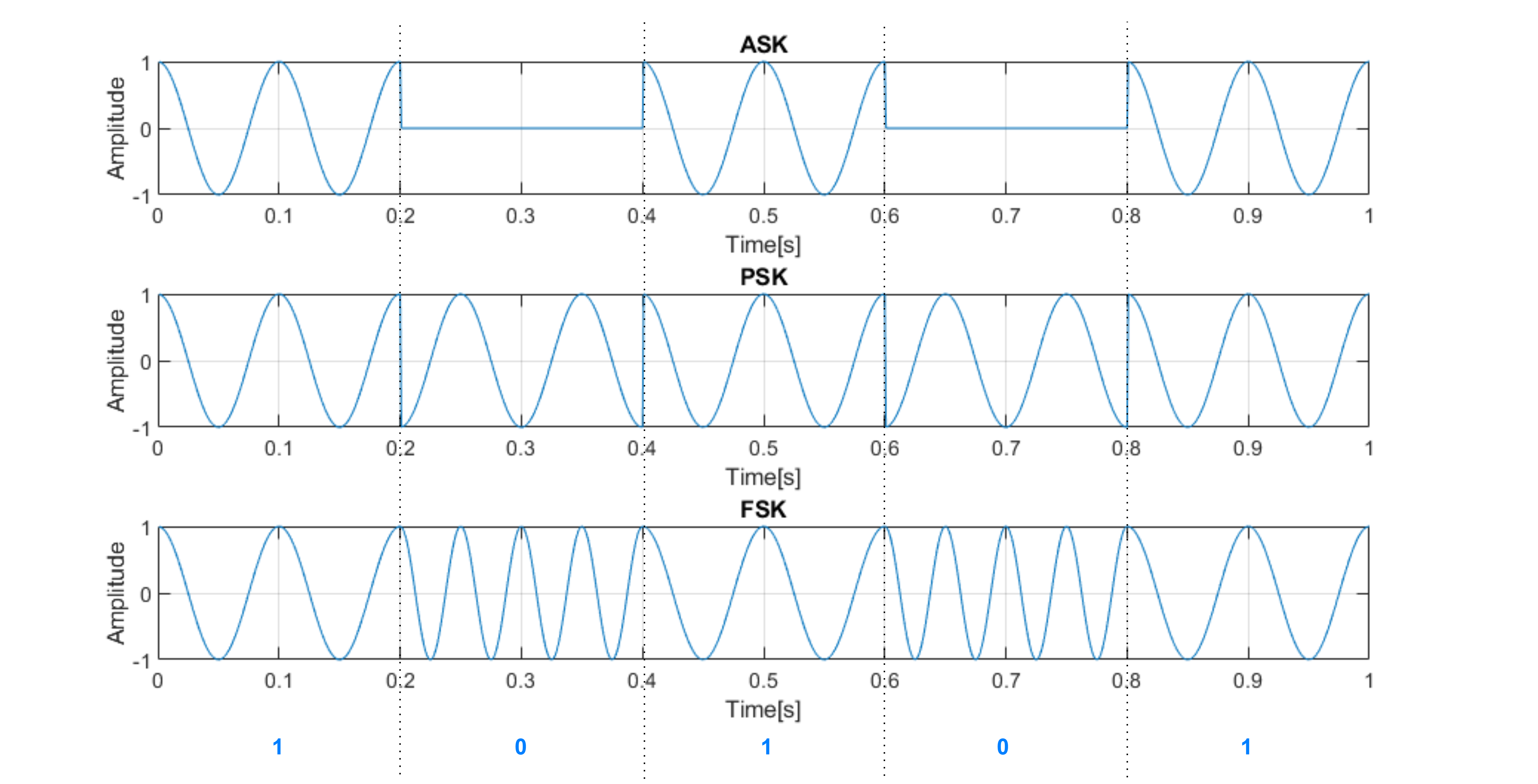
Fig. 2. An example of binary discrete modulations.
Quadrature Amplitude Modulation (QAM)
Each symbol can represent multiple bits of code. To encode \(b\) bits, \(2^b\) symbols are needed to represent all possible code combinations. The most basic example of QAM modulation is QAM 4. It uses 2 bits to encode \(2^2 = 4\) symbols. Base functions of QAM 4 modulation are; \(\phi_1 = cos(2 \pi f t), \phi_2 = sin(2 \pi f t)\). Modulated signal is obtained from base functions by using the expression \(s_i = s_i(1)\cdot\phi_1 + s_i(2)\cdot\phi_2\). Here, \(s_i(1)\) represent the in-phase (I) component of the symbol, and \(s_i(2)\) represents the quadrature (Q) component. This expression can also be rewritten in a complex form; \(s_i = Re[(s_i(1) + j s_i(2))\cdot(\phi_1 + j \phi_2)]\).
- 00:
\(s_1(1) = 1, s_1(2) = 1\)
\(s_1 = 1\cdot\phi_1 + 1\cdot\phi_2 = cos(2 \pi f t) + sin(2 \pi f t)\)
\(s_1 = Re [(\boldsymbol{1+j}) e^{-j 2 \pi f t}] = \sqrt{2} cos(2 \pi f t + \frac{\pi}{4})\)
- 01:
\(s_2(1) = -1, s_2(2) = 1\)
\(s_2 = Re [(\boldsymbol{-1+j}) e^{-j 2 \pi f t}] = \sqrt{2} cos(2 \pi f t + \frac{3 \pi}{4})\)
- 11:
\(s_3(1) = -1, s_3(2) = -1\)
\(s_3 = Re [(\boldsymbol{-1-j}) e^{-j 2 \pi f t}] = \sqrt{2} cos(2 \pi f t + \frac{5 \pi}{4})\)
- 10:
\(s_4(1) = 1, s_4(2) = -1\)
\(s_4 = Re [(\boldsymbol{1-j}) e^{-j 2 \pi f t}] = \sqrt{2} cos(2 \pi f t + \frac{7 \pi}{4})\)
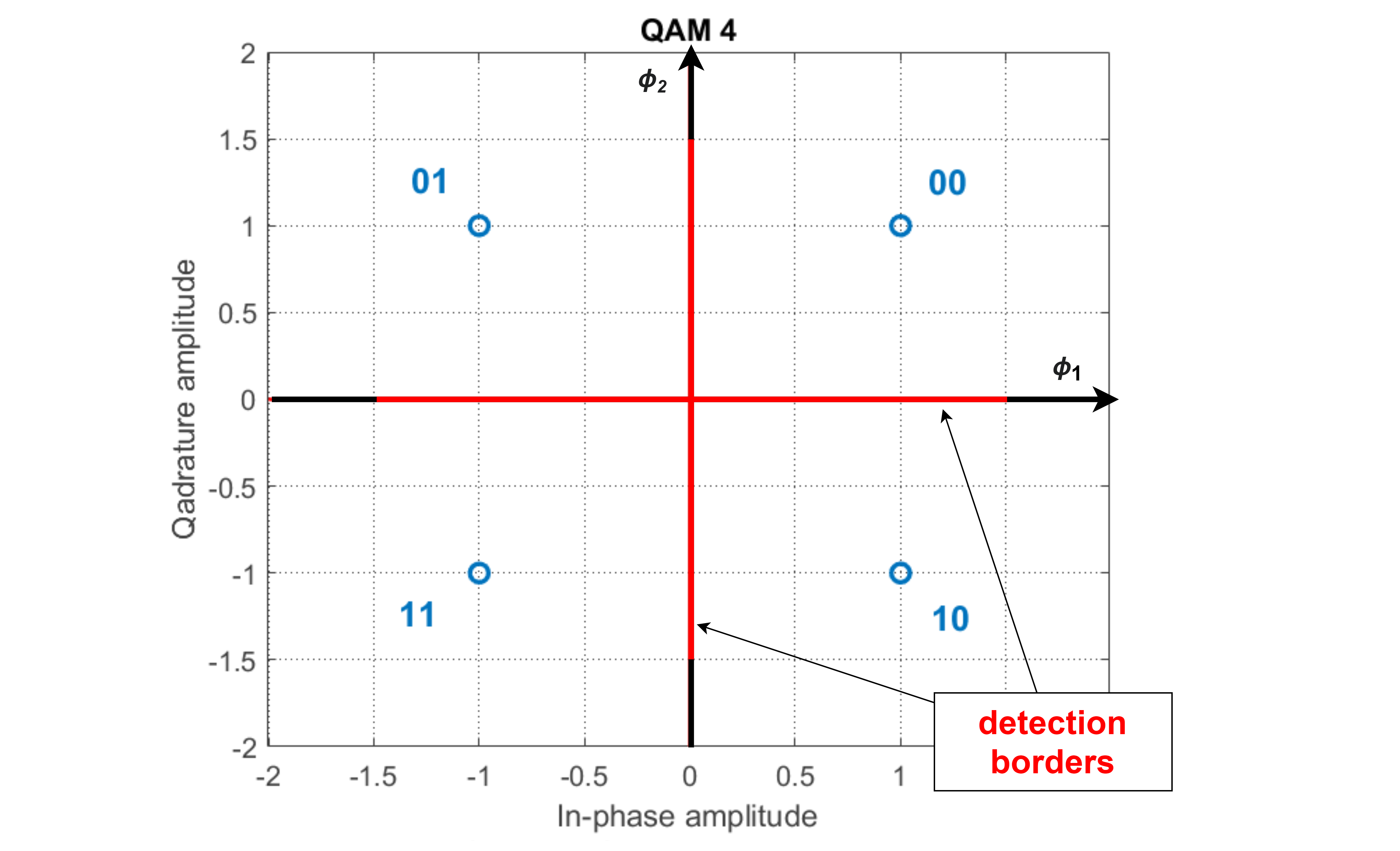
Fig. 3. 4-QAM constellation.
To perform demodulation, signal is translated in frequency and then filtered with low-pass filter; \(s_r = LP[s \cdot e^{j 2 \pi f t}]\). Demodulated signal values at given time are then mapped to the constellation to obtain wanted symbols. Symbol value is decided as the closest in mean square error (MSE) sense; \(min(\sqrt{(I_{sr}-I_m)^2 + (Q_{sr}-Q_m)^2}), m\in[1,M]\). Detection borders separate the areas where symbols have to fall in order to be detected correctly. Each symbol represents a binary value which then becomes a part of the output bitstream.
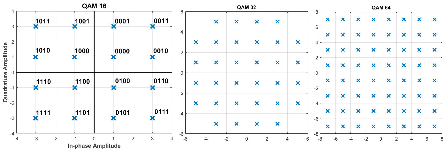
Fig. 4. QAM modulation can be performed for a larger number of bits.
Error Vector Magnitude (EVM)
If the signal properties degrade too much and the symbol falls into the area with different code representation, there is a possibility of wrong detection. The probability of the detection error increases almost linearly with the number of code combinations. The most common measure of modulation accuracy is Error Vector Magnitude (EVM). It is defined as the ratio of error magnitude and the largest symbol magnitude. If the received symbol is \(I_{sr} + jQ_{sr}\) and ideal symbol is \(I_{ideal} +jQ_{ideal}\), than the EVM is given as
EVM is usually measured for each symbol, and then averaged over the specified information block. It is also often expressed in percentage (%) or decibels (dB). Maximum EVM is specified in the communication system requirements and depends on the used modulation. For example, IEEE requirement states that the maximum value of EVM for systems using QAM 4 is -13dB.
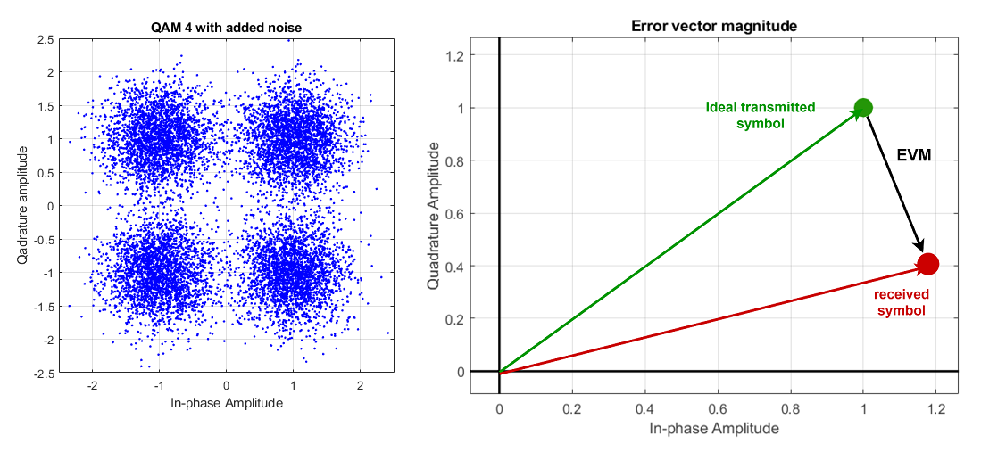
Fig. 5. Constellation of a 4-QAM signal with added white noise (left). EVM visualized (right).
Intersymbol Interference (ISI)
The impact of transmission path on discrete modulated signal is represented as various signal distortions, such as noise and intersymbol interference (ISI). One of the main cause of ISI is propagating the signal from transmitter to the receiver in multiple paths. This happens due to reflection from objects over the transmission path and it is called multipath propagation. In the real case, the envelope of the discrete modulated signal is not a rectangular window, but rather a function with smoother transitions, like sinc function or raised-cosine pulse. Each given symbol has some non zero components in the area of neighboring symbols. But it is very important that the symbol amplitude always stays zero in the detection point of other symbols. As the signals are distorted, they become wider in time and start to overlap with each other causing ISI.
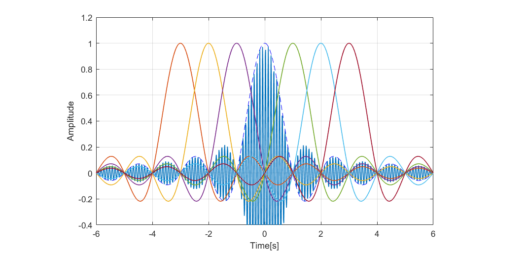
Fig. 6. Symbol envelopes in the ideal case without intersymbol interference.
Eye Diagram
The most intuitive way to observe noise and ISI is called the eye diagram. It is made by overlapping multiple symbol intervals on an oscilloscope. The eye diagram can indicate to the various deformations like clock dithering, noise, ISI and other non-linear effects.
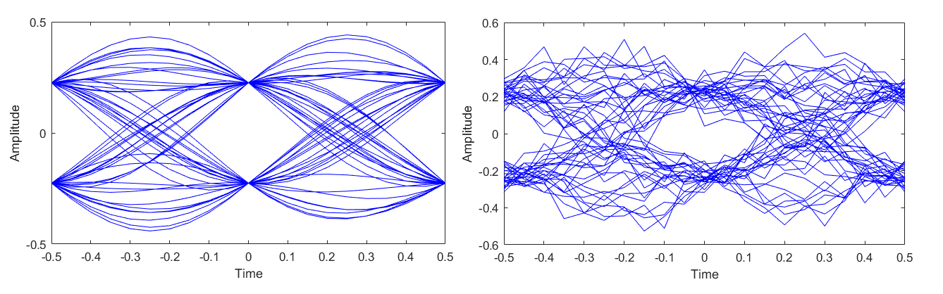
Fig. 7. An ideal eye diagram (left) and an eye diagram when noise and ISI are present (right).