Analog to Digital Conversion
Whenever a physical quantity should be processed in a computer system, it has to be represented in a form suitable for digital processing. Consider temperature measurements. A physical signal is measured on a thermometer and a value is read out from it. That way, a single temperature reading at a single moment is represented by a number of a given precision. We can say that the signal has been sampled and digitized. Let’s look more closely into these terms.
Sampling (and Hold)
At any given point in time, you can look at a thermometer and see the value it measures at that point in time. That value will change later on, so what you see when you look at it is a value that is correct only for a certain window of time. Reading out the value during that window is referred to as sampling. If you check the temperature every hour, we say you’re sampling at a frequency of f s = 1/ 3600 Hz = 0.28 mHz.
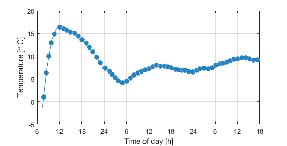
Fig. 1. A temperature graph taken across 3 days.
Let’s consider two issues about the measurement method that this graph presents:
- Sampling and holding time
It takes time for a temperature sensor to read out a value. Some sensors are quick in following rapid movements in temperature, while other take time to settle in. It is necessary to expose the measuring element to the physical quantity for a sufficient period of time for it to settle in. This is called sampling time.
Once the value has been picked up by the sensor, you may want to make sure the sensor displays the measured value long enough so you can read it. That period is called holding time.
- Seldom sampling
- Back to our ambient temperature graph, you will notice that in the morning of day 1 the temperature had been rising rapidly. If a temperature readout occurs every hour, it is impossible for the system to detect minor fluctuations in temperature. Higher sampling time allows us to pick up more frequent changes in the measured value. This is where the following theorem comes into play:
Nyquist-Shannon Sampling Theorem
Any signal represented by its frequency spectrum, populated up until frequency \(f_s/2\), can be faithfully reconstructed if it has been sampled by a sampling frequency of at least \(f_s\).
The frequency \(f_s\) is commonly referred to as Nyquist frequency, and it is determined by examining the signal that will be sampled. For instance, if an audio signal is fully contained within the 20 kHz bandwidth, a sampling frequency of 40 kHz will sufficient to faithfully represent the signal in the digital domain. (At least as far as sampling goes…)
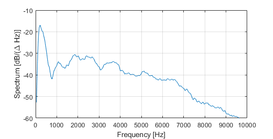
Fig. 2. A spectrogram of an audio sample.
The image in Fig. 2 represents a spectrogram of an audio sample containing male voice. Most spectral components reside at the lower end of the frequency range, and audio is virtually non-existent above 7 kHz. Therefore, a sampling frequency of 14 kHz is sufficient to sample this signal without losing relevant data.
Notice the axes of this image. The y axis is labeled in units of dB/(ΔHz). Here, dB is a ratio relative to the maximum value that can be represented in the notation used by the selected audio format. Since this is a spectral plot, the amplitude can only be presented across frequency. Hence, Hz -1. The (ΔHz) is used to emphasize that each point on the frequency plot represents an amplitude measured at multiple frequency points. The width of the measurement window is determined by the used time-to-frequency transformation method. In this case, it was a 1024-point FFT.
Frequency Axis
For any sampled signal, its frequency-domain representation resides on a finite frequency axis, as opposed to an infinite frequency axis for unsampled signals. Regardless of the sampling frequency, the frequency axis is defined in interval \([-\pi, \pi>\). Since the sampled signal is discrete, this frequency axis is periodic. Therefore, it is equally correct to rather define it on any other interval, \(2\pi\) in length, such as \([0, 2\pi>\) or \(<-\pi, \pi]\).
The physical interpretation of the frequency axis is evident when we map the interval \([-\pi, \pi>\) to \([-f_s/2, f_s/2>\).
Digitization
Each sample, taken at equally spaced time intervals 1/f s, now has to be read out and its value written down. At this point, we are still reading an analog value, e.g. the level of mercury on a thermometer. We can be infinitely precise in this process, and write down as many decimals as we’d like. Still, by assigning a value to each sample, we’ve performed digitization of the physical value.
The next step is to turn an infinitely precise value into something we can easily handle in a computer. This essentially boils down to rounding the numbers onto an arbitrarily defined discrete scale. This process is called quantization.
Typically, quantizers work in equidistant steps spread through the range of the binary number representation that is used in the computer. For instance, if we have 3 bits available, then 2 3 = 8 levels will be available for quantization. The distance between adjacent levels is typically referred to as 1 LSB.
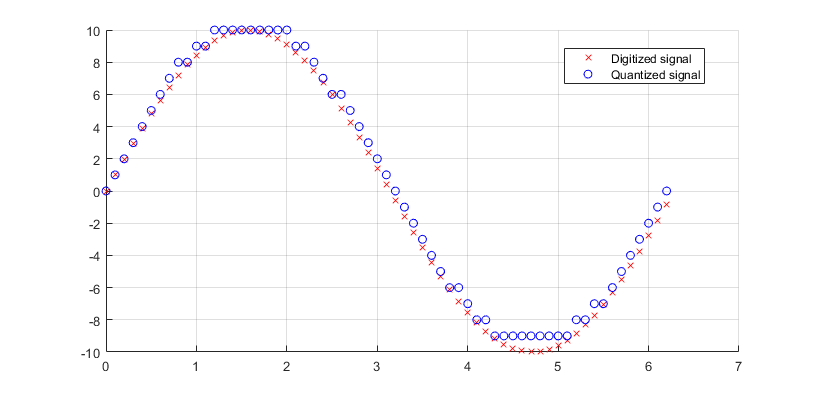
Fig. 3. An example of a digitized signal and its quantized counterpart.
The signal represented in red in Fig. 3 has been constructed as a digitized signal, with a sampling period of 0.1. We quantized this signal onto a digital scale defined by integers in range [-9,10]. Rounding method used was round-to-higher.
Quantization Noise
The issues of quantization, seen in this image, can be summarized by the term quantization noise. It is the offset between the value obtained after quantization, and the actual value of the digitized signal. For a sample above or below the quantization range, the quantization error is even higher, as the quantizer will have reached saturation with that signal.
This effect directly degrades the signal in further processing. For each combination of signal and quantizer, the degradation can be determined in terms of signal-to-quantization-noise ratio (SQNR). For a statistically random signal, and a quantizer with Q quantization bits available, SQNR can be approximated as